LAB 2 - Jesse and Shingo CS40/ENGR26
LAB DESCRIPTION
In this experiment, we implemented several primitive libraries that draw
basic shapes. We started by implementing the Image, which basically gives
us a canvas. Our canvas is a double pointer to an array of pixels, allowing
us to access a specific coordinate by canvas[row][col].
We next created the Point structure, which simply holds the coordinate
values. We used the Point structure to define Lines, which consists of
the starting point and the ending point. In order to draw a line, we
adopted the Bresenham's algorithm. The algorithm determines, for every
x-pixel, which y-pixel should be filled in to make the line appear
straight (when y / x > 1, we flip the x and y, then draw onto the canvas
accordingly). It can draw about 660,000 lines per second, with approximate
length of 102 pixels.
We also implemented Circle and Ellipse structures, using a similar method
as the line. We only actually draw 1/8 of the circle, we simply use the
reflection about the x-axis and/or y-axis to complete the circle. 1/8 of
the circle we draw is in the 3rd quadrant, because since the coordinate
is taken at the left-bottom corner, by drawing in the 3rd quadrant, we
ensure that colors we are filling in lay inside the circle. If we draw
in the 1st quadrant, then we will be adding to the outside of the boundary.
Ellipse is drawn in a simialr manner, except we had to do two parts of
4 reflected segments.
There is also the color class, but we never actually used it. We still
mainly used pixels, where RGB colors are 0 - 255. Colors are defined
as 0.0 - 1.0.
By changing the center of the circle and saving them in consecutive frames,
we were able to create an animation of a bouncing ball. We added 3 special
frames when the ball is at the bottom, where we draw an ellipse instead to
replicate the squishing of the ball.
We then used those primitives to draw a complicated image. It made us realize
how painful it is to draw individual lines, which led to the implementation
of the polygon class. It allows basic operations such as adding points and
drawing them, the polygon struct contains an array of points, maximum
number of points it can hold, and the number of points it currently holds.
Those last two fields help us prevent accessing nonexistent buckets of the
array, at the cost of flexibility.
TEAMWORK
In general tasks for this assignment were split evenly and usually shared between Jesse and Shingo. The following table lists the tasks and division of labor (although we really collaborated on everything):
| Task | Jesse | both | Shingo |
| Image Specification | | | X |
| Line | | X | |
| Dashed Line | | | X |
| Circle | | X | |
| Ellipse | | X | |
| Star Destroyer | X | | |
| Bouncing Ball | | | X |
| Polygon | | X | |
| writeup | X | | |
API
Libraries
Our graphics API includes a number of libraries for drawing objects and rendering them to the screen (using the Image library). Libraries 2-6 provide functionality for specifying primitives using mathematical coordinates and drawing them on an image. In general, you call a set function to define the primitive and then draw the primitive to an image (specified with the Image library). Keeping these two steps separate allows for the use of specialized set functionality such as drawing dashed lines or filled in shapes. It also allows one to use a point to define the center of a circle without actually having to draw that point to the screen.
Please note that much of the code was derived off code provided from other sources. Notably the image library uses code from PPMIO and the Line, Circle, and Ellipse code uses templates from the Hearn and Baker textbook provided by Maxwell.
- Image
- Point
- Line
- Circle
- Ellipse
- Polygon
State Variables
Notice that each library has a state variable associated with it. This is no accident. Each state variable holds the properties of some object. In the case of variables 2-6, these are things that can be drawn in the image object (state variable 1). Image specifies a drawing area and the properties associated with that and provides an interface with output using output types such as ppmIO.
- Image - a struct which includes data which can be accessed using imagename->data[row][column]. It also includes the number of rows and columns which can be accessed with imagename->rows and imagename->cols. Pixels or colors can then be assigned to each row/column location. Graphics routines access the state variables when they are passed in (when it is called). Aside from the interface specified in the lab requirements, the image library includes a few added features. The first is an inlined function called Image_access. The function takes the image and the current row and column as parameters and returns a boolean based on whether the point in question lies in the image to be drawn to the screen. This avoids issues with circles drawn outside of image coordinates etc. The other two functions Image_white and Image_black take an image file as input and fill it white or black. This is useful as a quick way to get a blank image for testing.
- Point - an array of 4 values x,y,z,h. The latter two are not yet being used. x and y specify the location the point should be drawn and can be passed in using pointname.val[i] with i=1,2,3,4. Graphics routines can access the point as a pointer.
- Line - This is a struct with two parameters, the starting point and the ending point. They can be specified using Point and passed in to Line_set, or specified as integer x,y coordinates using Line_set2D. Graphics routines access the state variables when they are passed in (when it is called). The line library includes the added extension Line_draw_dash which takes a line struct, image, pixel (color), and length in pixels to skip when drawing and draws a dashed line.
- Circle - a struct with radius defined as a double and the center using a Point. They can be passed in using Circle_set. These can be accessed using circlename->r and circlename->point[i]. Graphics routines access the state variables when they are passed in (when it is called)
- Ellipse - a struct with major axis ra and minor axis rb. The center is defined in the struct with a point. These can be passed in using Ellipse_set and accessed using ellipsename->ra, elllipsename->rb, ellipsename->pointname.val[i]. Graphics routines access the state variables when they are passed in (when it is called)
- Polygon - a struct containing an array of points which are vertices in the polygon, the max number of vertices the polygon can have num_vertex, and the current number of vertices it has curr_vertex. Points can be added using Polygon_add (which takes a poly struct and a point to add) or Polygon_add2D (for specifying points as integers). These return 0 on success or -1 if you cannot add any more points. The variables can be accessed using polygon->points[i], polygon->num_vertex, polygon->curr_vertex. The Polygon library includes two functions for drawing to an image. Poly_draw takes a poly struct, an image to draw to, and a pixel (color) and draws the polygon to the specified image. Poly_draw_dash draws a polygon in the same fashion but you can specify a skip length (the number of pixels to skip when drawing the lines of the poly). Finally, the Polygon library also includes two functions for clearing memory Polygon_clear and Polygon_free. Graphics routines access the state variables when they are passed in (when it is called)
COORDINATE SYSTEM ISSUES
In this class, creating computer graphics is bridging the gap between the medium of raster graphics which can be represented easily using pixels on screen and mathematics. Primitives such as circles and ellipses are drawn using mathematical formulas which means that using a mathematical coordinate system and translating that into pixel representation is imperative. This is especially true when 3D graphics are to be rendered.
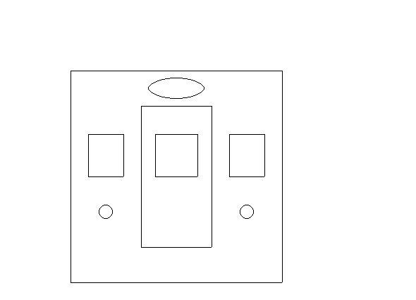
Required image demonstrating primitives
 |
To deal with coordinate system issues we modified the primitive code. For lineswe rendered all appropriate pixels except the last so that the theoretical length of the line matched the displayed length. This ensures boxes are the correct width and height and thus the correct volume.
Allowing users to specify the locations and sizes of primitives in theoretical space also presents the issue of rendering off the edge of the image displayed. This can have bad results. To deal with this we added a boolean image_Access function which takes theoretical coordinates and returns true or false based on whether the coordinates lie on the image. If they don't they're not rendered.
Circles and ellipses presented great challenges for ensuring they're the right theoretical size. To solve the problem, we had to draw them starting in the third quadrant rendering clockwise rather than the 1st. This ensures we are drawing pixels inside the theoretical boundaries.
Required image : Star Destroyer
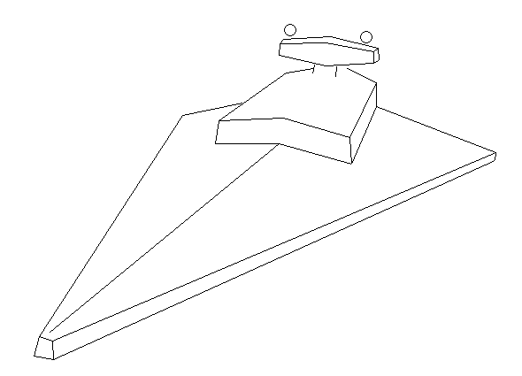 |
EXTENSIONS
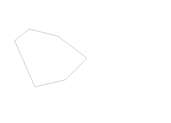
- Dashed Line
This is a function called Line_draw_dash which takes a line that has been set and draws it in dashed intervals whose lengths are set as a parameter. It is based on the same code used to draw a line.
- Bouncing Ball
The bouncing ball animation is a series of images called frames generated using a loop in which the position of a circle is changed according to the path of a bouncing ball under the force of gravity. The circle has also been changed to an ellipse whenever it contacts the bottom of the image to give the impression of a squashed ball.
- Polygon
Originally conceived to be able to draw shapes or our destroyer easily from a file of coordinates by inputing long arrays, this library now takes points as input using the function Polygon_add and doubles (like the original conception) using the function Polygon_add2D. These points are added to a structure containing an array of points. The polygon can be drawn to an image using a separate function which also allows the use of specialized functions such as ones for dashed polygons.