abstract.

In this lab various controllers were designed to control the angular position of a motor and flywheel system.  The input to the controller was a step corresponding to the desired final rotational position, and the output measured from the system was a voltage proportional to the rotational position.  We designed a lead controller and two different PID controllers to make the motor rotate twice and stop.

Phase-lead Controller Design

The motor transfer function for positional output is

Note that the system is type 1, meaning that there is no steady-state error to a step input.  As a result, the design of the controller would need a DC gain of 1.

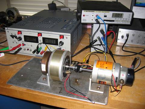
Generating the Bode plot for the uncompensated system gives the gain and phase margins shown below in Figure 1.

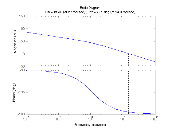
Figure 1. Gain and Phase Margins for Uncompensated System.

Since the gain margin is infinite, we do not worry about it.  Realizing the uncompensated phase margin is 4.31 degrees, we initially considered a phase-lead controller to increase the phase by 55 degrees for a compensated phase margin of 60 degrees.  However, since the addition of the controller also pushes up the gain slightly, we decided to design the controller to increase the phase by 58 degrees, because the uncompensated system gain corresponding 2 degrees phase was slightly below unity.  An approximate controller design was arrived at using the approximate equations below.

Therefore

Choosing  and applying the other equation, we obtain  and .  The transfer function of our phase lead controller is

The D.C. gain of this controller is 1.  We experimentally determined the controller gain 12.16k = 15 value to give us a nice and fast response; k equals 1.23.  This increases the D.C. gain above 1, which makes intuitive sense since a higher D.C. gain is needed to overcome the static and Coulomb friction in rotating the motor shaft.  The margins of the compensated open-loop system with k=1.23 are shown below in Figure 2.

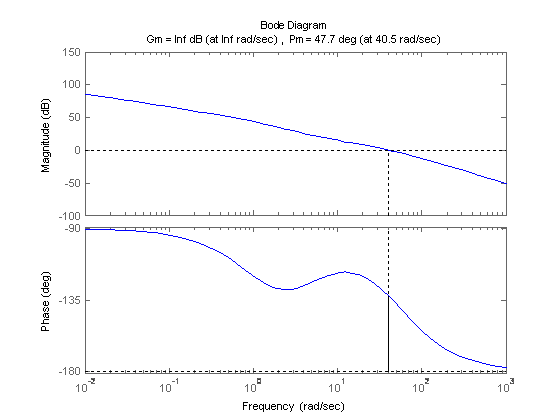
Figure 2.  Margins of open-loop Compensated system for k=1.

Using Matlab’s pole command, the closed-loop poles are at the following locations:

Since they are all in the left-half plane in the s plane, the system is stable.

A 2.4 volt step input, equivalent to two revolutions, is given to the closed-loop compensated system.  The simulation is shown below in Figure 3 along with the controller output.

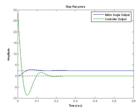
Figure 3:  Simulation of Phase-lead Design

As shown, the response is fairly 'good' in the sense that it settles quickly (around 0.1 seconds), and has decent overshoot.

Phase-lead Controller Revision

As discussed, the D.C. gain of the controller was slightly increased to account for the friction.  The theoretical and experimental responses are given below in Figure 4.

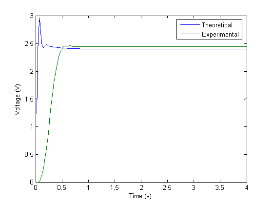
Figure 4. Theoretical and Experimental System Responses.

Note the apparent differences in the two responses.  The theoretical one gives some oscillations before settling to the correct final value.  The experimental response, however, spins up to the final value at a seemingly linear rate and settles there with no oscillations. 

The controller in real life experienced saturation, which accounts for the almost linear looking portion of the spin up graph.  The inflection at the beginning reminds us that the system is indeed third order with a closed-loop theoretical transfer function of

Again, we attempted to account for the static friction in the motor bearings simply by increasing the open-loop gain of the system.  The Simulink model including Coulomb friction and amplifier saturation is shown below.

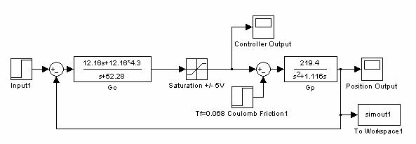
Figure 5. Theoretical Simulink Model (Lead) with Saturation and Coulomb Friction

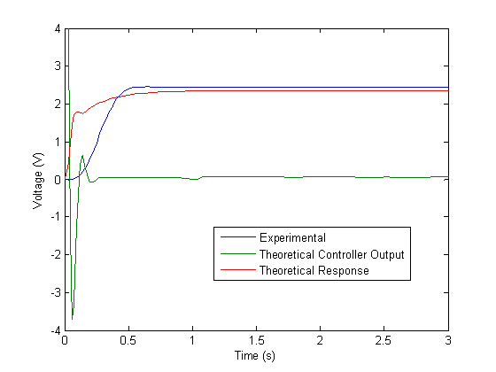
Figure 6.  Comparison of Simulink Model and Actual System

The effect of amplifier saturation is readily visible in the graph above.  The simulation resembles the actual response much better than before, and the remaining discrepancies probably result from an imperfect system model used in the simulations.

MATLAB Lead Controller Code

(note: relevant sections only)

% updated plant transfer function
Gp = tf([219.411], [1 1.116 0])
 
% lead controller tf
Gc = tf([a1 a0], [b1 1])
 
integrator1 = 0;
integrator2 = 0;
 
% apply a step input to the motor.
% to the motor leads.
 
while (Ain.SamplesAcquired<NumPts),
    j=Ain.SamplesAcquired;
 
    while(LastIndex==j),            %Wait for next datum.
        j=Ain.SamplesAcquired;
    end
    if ((j-LastIndex)~=1),          %Make sure no data was missed.
        disp(sprintf('Warning, datum skipped: %d, %d',LastIndex,j));
    end
    InData=peekdata(Ain,j);         %Retrieve most recent datum.
 
    if (t(j)<0),        %If during PreSample, output 0.
        PosVoltage(j)=0;
    else                %Else, do control algorithm
        PosVoltage(j) = InData(j);
    end
 
    % calculate the error signal
    errsig(j) = InputVal - PosVoltage(j);
 
    % run the integrators
 
    % integral( IN(t)*dt )
    if (j>1)
        integrator1 = integrator1 + (errsig(j)+errsig(j-1))*DT/2;
    else
        integrator1 = integrator1 + errsig(j)*DT/2;
    end
 
    % integral( OUT(t)*dt )
    if (j>2)
        integrator2 = integrator2 + (output(j-1)+output(j-2))*DT/2;
    else
        integrator2 = 0;
    end
 
    % apply the output of the three controllers
    output(j) = a1/b1*errsig(j) + a0/b1*integrator1 - 1/b1*integrator2;
 
    if (output(j) > 5)
        output(j) = 5;
    elseif (output(j)<-5)
        output(j) = -5;
    end
 
    putsample(Aout, output(j));
 
    LastIndex=j;
end
 
% turn off the motor
putsample(Aout,0);

PID Controller Design

We used a 3-stage fuzzy logic PID to control our system. The k_p, k_i and k_d values were changed depending on the current status of the error signal. For error values above a certain percentage of the desired output (in our case it was 30%) we used a large k_p constant to drive the system as hard initially to get up towards the desired final value as quickly as possible.  This results in saturation of the amplifier.  For values in the second stage (in our case 30% - 10% of the desired output) we used a controller that tended to slow down the motor by having a relatively large k_d while lessening the k_p term.  If we kept using the controller from the last stage, the system would overshoot substantially and it would take the motor a lot of time to settle.  In the last stage, we decreased k_d to once again speed up the system.  We made the design decision to make sure that we never revisited a controller stage more than once so that it would naturally progress from stage one up to three.

We couldn’t come up with a three-stage PID controller that worked better than the lead controller we designed.  There were a couple of problems we faced in the design process. Firstly, our design was dependant on the desired output.  If the desired output was large, then the controller would work slightly better, but if the output was small, we couldn’t speed it up enough in the first stage which affected the performance in the latter stages.  Similarly, if the desired output was large, then the system was too fast.

We tried to adjust the boundaries of the stages in various ways. We first tried static values (not percentages of the desired output) but that was problematic for desired outputs that were close to the boundaries or that were in the second or final stage.  Our second approach of defining boundaries as percentages of the output was better but we still couldn't come up with good values.  In the overall design, there were too many parameters that we could adjust (k_p, k_d, k_i values as well as stage boundaries) but we couldn't come up with a design that was better than the lead design consistently (for some values it performed better, but it was very slow for others).

Figure 7 gives some sample output from the system under our PID control.  In particular, notice the D/A output which has two distinct jumps which correspond to the changing of stages in our fuzzy logic controller.

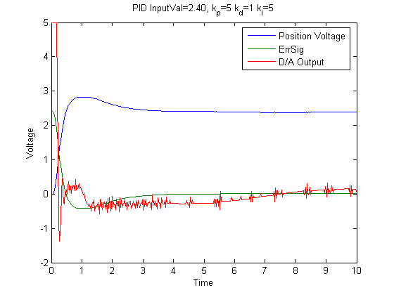
Figure 7:  Sample of PID control