Abstract

In this laboratory experiment, a DC motor was controlled by proportional and integral controllers.  After the motor was allowed to spin up to steady state, a load motor was enabled.  The proportional controller was not able to recover from the perturbation, while the integral controller was able to.  The integral controller also achieved a zero error signal, while the proportional controller could not because then the motor would have stopped rotating. The simulated responses of the system to the step inputs were calculated in MATLAB and compared to the experimental data.  The experimental and theoretical results compared very favorably, confirming the accurate characterization of the motor system in Lab 2.

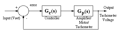
Transfer Functions of the Motor System

The motor system is given in the following block diagram. 

For the proportional controller, the motor system transfer function, where G_C = k_p is given by

For integral control, the motor system transfer function is

Graphs of Experimental Data

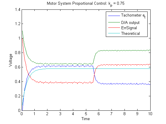
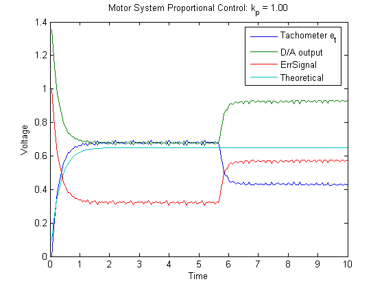
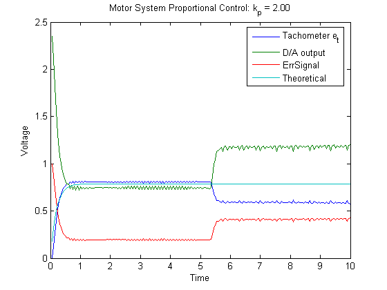
The theoretical responses shown in the graphs below were calculated in MATLAB using the tf and step commands.  The disturbance by shorting the load motor wires was applied approximately in the middle of the sampling time, allowing the motor to achieve steady state again after the disturbance.

Proportional Control

Graph 2A. Proportional k_p=0.75

Graph 2B. Proportional k_p=1

Graph 2C. Proportional k_p=2

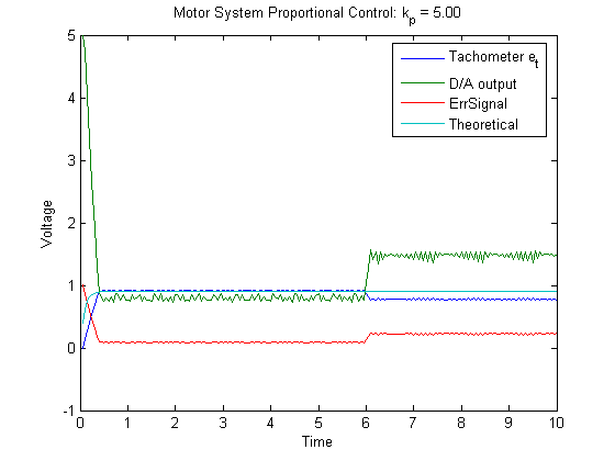
Graph 2D. Proportional k_p=5

Integral Control

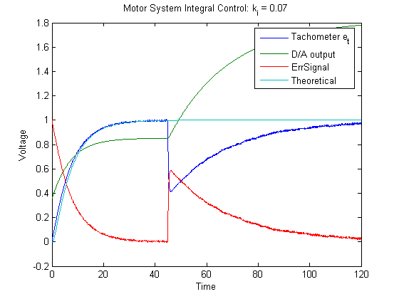
Graph 2E. Integral k_i=0.067

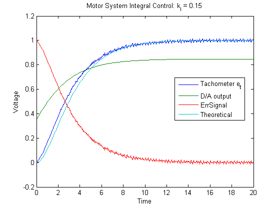
Graph 2F. Integral k_i=0.151

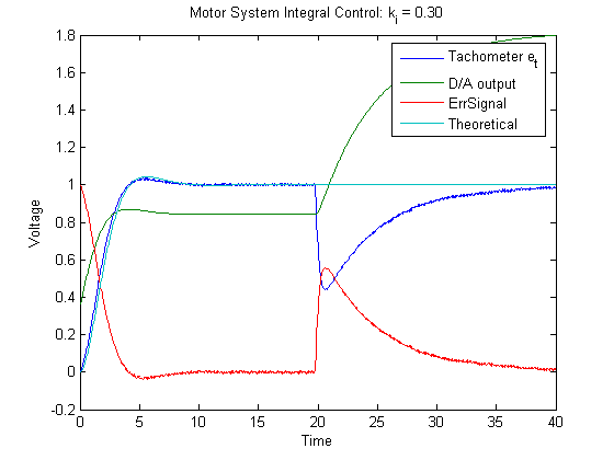
Graph 2G. Integral k_i=0.302

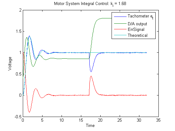
Graph 2H. Integral k_i=1.677

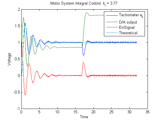
Graph 2I. Integral k_i=3.773

Steady State and Time Constant for Proportional Control

For the proportionally controlled motor system, the time constant and steady state (sŕ0) for a unit step values are found by inspection of the transfer function given previously.

 , 

Various time constants and steady state values are given in Table 4A below.

Table 4A. Theoretical and Experimental Time Constants and Steady State Values.

* The experimental response no longer is in the shape of a normal exponential because the motor is ramped up too quickly by the large k_p values.

Damping Ratio and Natural Frequency for Integral Control

For the integral controller, the 2^nd order damping ratio and natural frequency are given by

 ,

To calculate experimental values of and , we use the equations given below.  We define  as the percent overshoot.

Looking at the graphs, we can calculate  from measuring the period of damped oscillation on the graphs.  We use the following equation to obtain the natural frequency .

Table 5A. Theoretical and Experimental Damping Ratios and Natural Frequencies

* For , the characteristic equation of the transfer function factors into two real roots, so there is no oscillation.  As a result, the damping ratio  and natural frequency  do not apply.

Extension

We created a PID controller in simulink as shown in F1 below.  For the purposes of this lab, we set k­_d to zero to create a PI controller and explored the optimal system response which we define to be when =.707.

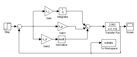
Figure F1. Simulink block diagram for a PID controller.

The characteristic equation of the system with a PI controller in place can be shown to be:

Imposing our constraint of =.707 reveals the following relationship between k_i and k_p:

Choosing a few particular values for k­­_I and k_p yields the results shown in Figure F2 below.

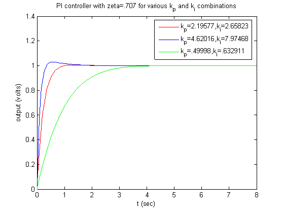
Figure F2. PI controller system response with =.707 for selected k_p and k_i.

Depending on the value of k_i, the natural frequency of the system changes, making the system faster or slower.  Increasing the system speed by choosing a higher value of k_i comes at the expense of greater overshoot as seen in Figure F2.  The ideal balance of system speed and overshoot is dependent on the particular application of the system.

Points of Interest / Conclusion

From the lab, the basic difference we found for the two different controllers is the impact each has on the steady state error of the system response.  As shown from graphs 2A-2D, the steady state error is not zero corresponding to the proportional control system.  Graphs 2E-2I, corresponding to the integral control, clearly shows that the system steady state error approaches zero.  The fundamental difference between the two controllers is that the integral control integrates the steady state error, thus giving the system a non-zero error input to drive the system.  Having the system driven serves to allow it to steadily reduce the error until it is zero.  Without the integrating term (effectively having a proportional control), the steady state error can be non-zero as mentioned.

The integral controller also added a new response feature to the system by making the system response second order.  Depending on the value of, the value of of the system is determined.  When less than 1, the system response is underdamped and exhibits a decaying oscillation that approaches the final value.  When is greater than 1, the system is overdamped with a response that has no overshoot approaching the final value.  equals 1 is the case of critical damping when the response approaches the final value the quickest with no oscillations.  The system error displays the same response characteristic shown in graphs 2E-2I.

The motor was shorted out during the latter part of each trial run by pulling a switch, and the responses are shown in the graphs found in section 2.  As expected, the proportional control system reaches its new steady state value with the addition of the load, but the steady state error does not approach zero.  In contrast, the steady state error of the integral control system approaches zero.

For the proportional control, when the k values were too high (k > 1) the D/A output ramped, thus causing the tachometer voltage to do the same.  The theoretical and experimental system responses are no longer similar to one another. (Refer to Graph 2C and 2D)

The theoretical system response of the system had the effects of Coulombic friction included, and matched the experimental responses quite well as shown in the graphs.  The time constants, damping ratios, natural frequencies, and steady state values matched quite well as shown in Tables 5A and 4A. 

The coupling component on the motor shaft snapped during the middle of the lab.  We replaced the malfunctioned part with one from another apparatus, and continued the lab.  The fix should not greatly affect the performance of the motor and thus our results. 

We had to be careful with our desired voltage outputs; since the bipolar operational power supply / amplifier cannot output a voltage greater than 36 volts (or ~6 Amps) we maintained a low desired output voltage to ensure we did not saturate the amplifier.

MATLAB SCRIPTS FOR INTEGRAL CONTROLLER

function [] = integral(k_i, SampleTime)
% runs the motor, plots some graphs, and saves some data
% usage: intergral(k_i, SampleTime)
%
% Engineering 58 Lab 3
% David Luong, Mark Piper, akader, Aron Dobos
% Set up sampling parameters
             %Clear the display
SampleFreq=20;         %Sampling Frequency
%SampleTime=25;           %sampling time (seconds)
if SampleTime*SampleFreq >= 2000
    return
end
NumPts=SampleFreq*SampleTime;             %Number of points in run (<=2000).
PreSample=0;           %Number of points before control
                        %  algorithm runs (this generates
                        %  baseline data);
InChan=0;               %Input channel to use on DAQ board
OutChan=0;              %Output channel to use on DAQ board
DT=1/SampleFreq;        %Sampling Interval
%Setup the input channel
%You shouldn't need to change this.
Ain = analoginput('nidaq');
Ain.SampleRate=SampleFreq;
Ain.SamplesPerTrigger=NumPts;
Ain.InputType='SingleEnded';
Ain.BufferingConfig=[1  2000];
Ain.TransferMode='Interrupts';
addchannel(Ain,InChan);
%Setup the output channel
%You shouldn't need to change this.
Aout = analogoutput('nidaq');
addchannel(Aout,OutChan);

%%%%%%%%%%%%%%%%%%%%%%%%%%%%%%%%%%%%%%%%%%%%%%%%%%%%%%%%%%%
%%%%%%%% Predefine any arrays to make loop quicker %%%%%%%%
%%%%%%%%%%%%%%%%%%%%% Change as needed %%%%%%%%%%%%%%%%%%%%
%%%%%%%%%%%%%%%%%%%%%%%%%%%%%%%%%%%%%%%%%%%%%%%%%%%%%%%%%%%
TachData=zeros(NumPts,1);
DtoAData=zeros(NumPts,1);
ErrSig=zeros(NumPts, 1);
%%%%%%%%%%%%%%%%%%%%%%%%%%%%%%%%%%%%%%%%%%%%%%%%%%%%%%%%%%%

%Define Time Vector (time=0 after PreSample is done)
t=((1:NumPts)-PreSample)*DT;
LastIndex=0;
start(Ain);

% turn off the motor initially - the controller will turn it on as
% necessary
putsample(Aout,0); 

% apply a step input to the motor.  This applies 2.5*7.2 = 18 V
% to the motor leads.
integrator = 0;

% integrator controller constant
%k_i = 3.773;
% this is the desired tachometer voltage (e_t, the output)
DesiredTachVoltage = 1;
while (Ain.SamplesAcquired<NumPts),
    j=Ain.SamplesAcquired;
    while(LastIndex==j),            %Wait for next datum.
        j=Ain.SamplesAcquired;
    end
    if ((j-LastIndex)~=1),          %Make sure no data was missed.
        disp(sprintf('Warning, datum skipped: %d, %d',LastIndex,j));
    end
    InData=peekdata(Ain,j);         %Retrieve most recent datum.
    if (t(j)<0),        %If during PreSample, output 0.
        TachData(j)=0;
    else                %Else, do control algorithm
        TachData(j) = InData(j);
        ErrSig(j) = DesiredTachVoltage - TachData(j);
        err_old = 0;
        if (j-1>0)
            err_old = ErrSig(j-1);
        end
        integrator=integrator+(ErrSig(j)+err_old)*DT/2;
        DtoAData(j) = k_i * integrator;
        % adjust for coulomb friction with equation R/(A*k_t)*t_f
        DtoAData(j) = DtoAData(j) + 0.3558;
        if (DtoAData(j) > 4.995),
            DtoAData(j) = 4.995;
        elseif (DtoAData(j) < -5),
            DtoAData(j) = -5;
        end
        putsample(Aout, DtoAData(j));
    end
    %%%%%%%%%%%%%%%%%%%%%%%%%%%%%%%%%%%%%%%%%%%%%%%%%%%%%%%%%%%
    LastIndex=j;
end
% turn off the motor
putsample(Aout,0); 
%Free up any memory that we used.
delete(Ain)
clear Ain
delete(Aout)
clear Aout
sys = DesiredTachVoltage*tf([2.063*k_i],[1 1.116 2.063*k_i]);
[TheoreticalStep n] = step(sys, t);
plot(t,TachData, t, DtoAData, t, ErrSig, t, TheoreticalStep)
legend('Tachometer e_t', 'D/A output', 'ErrSignal', 'Theoretical');
xlabel('Time');
ylabel('Voltage');
title(sprintf('Motor System Integral Control: k_i = %.2f', k_i));
filename = sprintf('integral_ki_%.2f.bmp', k_i);
print('-dbitmap', filename);
filename = sprintf('integral_ki_%.2f.mat', k_i);
save(filename,'t','TachData', 'DtoAData', 'ErrSig', 'TachData', 'TheoreticalStep')
beep
disp('Data Aqcuisition done.');

MATLAB SCRIPTS FOR PROPORTIONAL CONTROLLER

function [] = proportional(k_p, SampleTime)
% runs the motor, plots some graphs, and saves some data
% usage: proportional(k_p, SampleTime)
%
% Engineering 58 Lab 3
% David Luong, Mark Piper, akader Kader, Aron Dobos
%
% Set up sampling parameters
SampleFreq=20;         %Sampling Frequency
%SampleTime=10;           %sampling time (seconds)
if SampleTime*SampleFreq >= 2000
    return
end
NumPts=SampleFreq*SampleTime;             %Number of points in run (<=2000).
PreSample=0;           %Number of points before control
                        %  algorithm runs (this generates
                        %  baseline data);
InChan=0;               %Input channel to use on DAQ board
OutChan=0;              %Output channel to use on DAQ board
DT=1/SampleFreq;        %Sampling Interval
%Setup the input channel
%You shouldn't need to change this.
Ain = analoginput('nidaq');
Ain.SampleRate=SampleFreq;
Ain.SamplesPerTrigger=NumPts;
Ain.InputType='SingleEnded';
Ain.BufferingConfig=[1  2000];
Ain.TransferMode='Interrupts';
addchannel(Ain,InChan);
%Setup the output channel
%You shouldn't need to change this.
Aout = analogoutput('nidaq');
addchannel(Aout,OutChan);

%%%%%%%%%%%%%%%%%%%%%%%%%%%%%%%%%%%%%%%%%%%%%%%%%%%%%%%%%%%
%%%%%%%% Predefine any arrays to make loop quicker %%%%%%%%
%%%%%%%%%%%%%%%%%%%%% Change as needed %%%%%%%%%%%%%%%%%%%%
%%%%%%%%%%%%%%%%%%%%%%%%%%%%%%%%%%%%%%%%%%%%%%%%%%%%%%%%%%%
TachData=zeros(NumPts,1);
DtoAData=zeros(NumPts,1);
ErrSig=zeros(NumPts, 1);
%%%%%%%%%%%%%%%%%%%%%%%%%%%%%%%%%%%%%%%%%%%%%%%%%%%%%%%%%%%

%Define Time Vector (time=0 after PreSample is done)
t=((1:NumPts)-PreSample)*DT;
LastIndex=0;
start(Ain);

% turn off the motor initially - the controller will turn it on as
% necessary
putsample(Aout,0); 

% apply a step input to the motor.  This applies 2.5*7.2 = 18 V
% to the motor leads.
% proportional controller constant
%k_p = 2;
% this is the desired tachometer voltage (e_t, the output)
DesiredTachVoltage = 1;
while (Ain.SamplesAcquired<NumPts),
    j=Ain.SamplesAcquired;
    while(LastIndex==j),            %Wait for next datum.
        j=Ain.SamplesAcquired;
    end
    if ((j-LastIndex)~=1),          %Make sure no data was missed.
        disp(sprintf('Warning, datum skipped: %d, %d',LastIndex,j));
    end
    InData=peekdata(Ain,j);         %Retrieve most recent datum.
    if (t(j)<0),        %If during PreSample, output 0.
        TachData(j)=0;
    else                %Else, do control algorithm
        TachData(j) = InData(j);
        ErrSig(j) = DesiredTachVoltage - TachData(j);
       % DtoAData(j) = k_p*(DesiredTachVoltage + ErrSig(j) + 0.6415)/1.86; % + (DesiredTachValue+0.6415)/1.86;
        DtoAData(j) = k_p * ErrSig(j);   
        % adjust for coulomb friction with equation R/(A*k_t)*t_f
        DtoAData(j) = DtoAData(j) + 0.3558;
        if (DtoAData(j) > 4.995),
            DtoAData(j) = 4.995;
        elseif (DtoAData(j) < -5),
            DtoAData(j) = -5;
        end
        putsample(Aout, DtoAData(j));
    end
    %%%%%%%%%%%%%%%%%%%%%%%%%%%%%%%%%%%%%%%%%%%%%%%%%%%%%%%%%%%
    LastIndex=j;
end
% turn off the motor
putsample(Aout,0); 
%Free up any memory that we used.
delete(Ain)
clear Ain
delete(Aout)
clear Aout
sys = DesiredTachVoltage*tf([2.063*k_p],[1 1.116+2.063*k_p]);
[TheoreticalStep n] = step(sys, t);
plot(t,TachData, t, DtoAData, t, ErrSig, t, TheoreticalStep)
legend('Tachometer e_t', 'D/A output', 'ErrSignal', 'Theoretical');
xlabel('Time');
ylabel('Voltage');
title(sprintf('Motor System Proportional Control: k_p = %.2f', k_p));
filename = sprintf('proportional_kp_%.2f.bmp', k_p);
print('-dbitmap', filename);
filename = sprintf('proportional_kp_%.2f.mat', k_p);
save(filename,'t','TachData', 'DtoAData', 'ErrSig', 'TachData', 'TheoreticalStep')
%%%%%%%%%%%%%%%%%%%%%%%%%%%%%%%%%%%%%%%%%%%%%%%%%%%%%%%%%%%
beep
disp('Data Aqcuisition done.');