where
 now since R = 0.
Plugging in
 , we get
For convenience, let the quantity

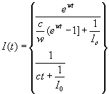
So the solution for I is

From that solution, as t -> infinity,

So

The key difference when modeling a recurring epidemic is that when
infected people recover, they become susceptible again (rather than
immune or dead), such as is the case with the common cold. With this
modification, the previous equations become

where  now since R = 0.
Plugging in  , we get

For convenience, let the quantity

So the solution for I is

From that solution, as t -> infinity,

So

This model therefore gives the same equilibrium position as the chicken
pox model, the non-recurrent epidemic model. This fact seems to suggest that
the recurrence of a disease does not affect its equilibrium position, which
seems illogical. The difference here is that the population of infected people
in the two cases is not the same. In the recurrent epidemic, the same number
of total people are infected at the equilibrium, but some of them have been
infected one or more times before. The non-recurrent epidemic infects more
different people, but still the same total number.
A factor that is not considered by the non-recurrent model is that of
vaccination. Each person who is vaccinated against the disease is effectively
removed from the population being modeled. Then, though the equilibrium value
does not change fractionally, the total population is smaller, so the total
number of people infected at equilibrium is smaller.
(Ref 3)
The first mathematical model of the AIDS epidemic was published in 1986
by Anderson et al. The most serious characteristic of the virus was then
considered to be the length of time during which noticeable symptoms had not
yet developed. This model therefore measured the rate at which HIV-infected
persons acquired AIDS.
In the population being considered, initially all people have HIV but have
not yet acquired AIDS. It is assumed, however, that all members of the
population will eventually acquire AIDS.
We will let the fraction of the population of persons with HIV but no AIDS
symptoms be described by H(t) and the fraction of that with AIDS by A(t).
Then

where c(t) is the rate of conversion between HIV and AIDS.
In order to fulfill the assumption that all members of the population acquire
AIDS, A(t) must be an increasing function, so A must be positive. c(t) must
therefore be positive. We will assume that c(t) = ct where c is a positive
constant.
Solving the differential equations yields

We can then see that as  ,
and
,
and  ,
,
 as assumed. The best fit value of c
has been determined statistically to be approximately 0.237 per yr.
This model, though useful for determining the expected latency period of
HIV, does not give any information about the spread of HIV throughout an
uninfected population. To be more helpful for public health officials and
medical professionals, models of infection rates would need to be developed.
This is just what Andersons revised model did.
(Ref 3)
Andersons revised model of the HIV epidemic was published in 1989.
Due to the status of the epidemic at the time, it only considers a male
population.
A constant immigration rate B of susceptibles is assumed. The size of the
total population is given by N(t). X(t) gives the number of susceptibles at
any time. Y(t) gives the number of infectious males. A(t) gives the number
of AIDS patients. Z(t) gives the number of uninfectious seropositives. This
last portion of the population includes those who have isolated themselves
from the rest of the population.
Without the presence of any infection (no AIDS deaths), the equilibrium
population is assumed to be  ,
where u is the rate of natural death. d is taken to be the rate at which
AIDS patients die.
  is defined
to be the probability of acquiring infection from a randomly chosen
partner, where b is the transmission probability. v is defined as the rate
of conversion from HIV to AIDS, and c is the average number of sexual
partners per person.
 is defined as the proportion
of seropositives who are infectious.
Finally, it is assumed that there is a uniform mixing of the populations.
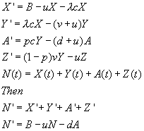
The rates of change of each segment of the population can then be modeled:

If the number of secondary infections resulting from a primary infection is
greater than one, an epidemic ensues. The threshold value would then be bc/v.
Making the substitution

we get a nonlinear system. In order to find the solution to the system,
each equation can be linearized by making the substitution X = X* + x (and
the equivalent for each variable), where X* represents the nominal value
and x the incremental value. The operating point can be found by setting all
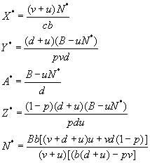
incremental values to zero. After much algebra, one gets this set of values:

Then, one uses the Taylor series approximations of the nonlinear elements of
the equations to linearize them.
Taylor series expansion:

Next, one substitutes and subtracts off all nominal values to obtain equations
in terms of only incremental values. These equations can then be solved to find
the time-varying solution.
In this case, it is found that X, Y, Z, A, and N are oscillatory and tend
towards zero. (Ref 3)
It is important to note that, originally, all of the constants used were based
on case studies of HIV patients and data collected from several cities in the
United States. These constants can therefore be adjusted with the insight of
additional data for a more accurate model.