Image Mask
We created the image mask based on the assumption that the camera formed circular images in the center of the image. This turned out to be not exactly accurate (some of the images had different centers than the others). To account for this, we chose to mask off more of the image than is technically necessary, by only considering the circle centered at the center of the image, with a slightly smaller radius. Additionally, we needed to make the radius slightly smaller to account for the gray ring with LEDs that the lens put in the image. In total, our circle's radius is 91% of the "radius" of the image (1/2 the length of the shorter dimension), centered at the center of the image. We settled on the 91% figure by comparing masking results across the images, and picking the largest value that entirely excluded the light gray ring in all the images.
Thresholding Techniques
In addition to being able to specify an image-wide threshold value at the command line (all pixels with intensities > the specified threshold are counted as sky, and everything else becomes canopy), our program can compute thresholds automatically using the ISODATA algorithm. Specifying -1 on the command line will cause our program to ignore the user-specified threshold.
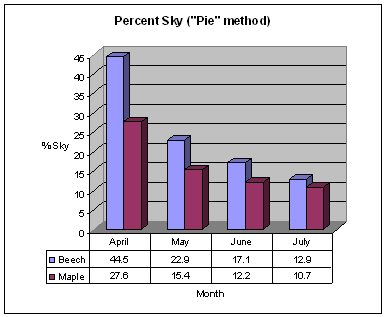
ISODATA thresholds are computed for each of the "regions" of the image. The number of regions is defined as a preprocessor macro near the top of ppmmain.c. Setting REGIONS to 1 will accomplish the same thing as having no regions (as in task 4). Initially we divided the region into concentric circles with equal widths, but found that in some images, this caused undesired results (specifically, in norwayMaple-June-1W.pgm) a large portion of the area near the edge of the circle was counted as sky, though very little of that area is, in fact, sky. Because of this, we choose to also implement another regioning method, which divides the image into wedge-shaped regions. Entering 0 as the 4th command line argument causes ppmmain.c to use the "pie" method; entering 1 causes it to use the "circle" method (see figures below). One peculiarity of the "pie" method is that the regions it forms are actually bowtie-shaped, as a side-effect of the range of the arctangent function. With some minor modifications, we could correct for this condition, but we ran out of time.
Regardless of which method is chosen, the ISODATA algorithm is computed for
the histogram of each region of the image. During the first scan of the image,
each pixel is identified uniquely with a region (using the methods pie_region() and concentric_region()).
The region is used as an index into the first field of the two-dimensional
histarray (long histarray[REGIONS][256]), which contains "buckets"
for each of the intensities possible in the PGM, for each region. The ISODATA
algorithm is run on each of the regions in the image. Within each, a unique
threshhold is chosen, which is then used to compute sky and canopy counts
for that region only. The threshold of the previous region is
used as the starting threshold of the ISODATA algorithm for the next region
(the first region has a default starting threshold of 128). The only other
change to the ISODATA algorithm was to divide the variable canopymean by
canopycount (and skymean by skycount)
before comparing, since without this step, canopymean and skymean are totals,
not means.
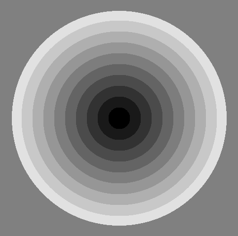 Regions in "circle" method |
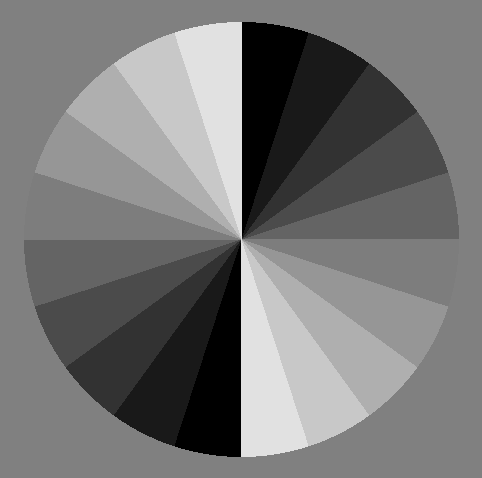 Regions in "pie" method |
Calculating Percent Sky
If REGIONS is greater than 1, we calculate the total number of sky pixels (the number of sky pixels per region is calculated, and then added to the total), and is then divided by the number of pixels in the regions we're considering (inside the circle). Setting REGIONS to 1 does essentially the same thing, except there is only 1 region which encompasses the entire area within the circular mask.
 |
 |
 |
|
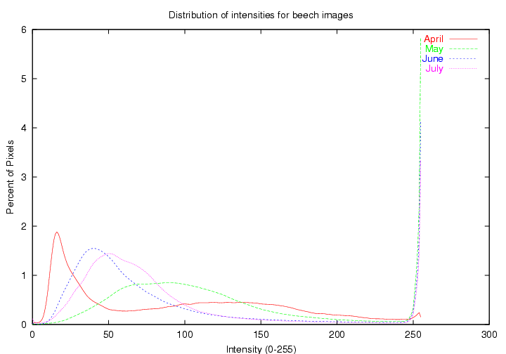 Intensity histogram for beech tree images |
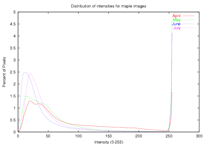 Intensity histogram for norway maple images |
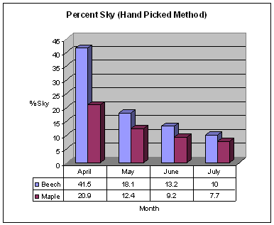
For the "Hand Picked" method, we chose thresholds by averaging the intensity of a point midway up and across the "main trunk" in each image with a point of average intensity in the sky. Below are the actual threshold values used:
| Beech | Maple | |
|---|---|---|
| April | 41.5 |
20.9 |
| May | 18.1 | 12.4 |
| June | 13.2 | 9.2 |
| July | 10.0 | 7.7 |
Sample Images
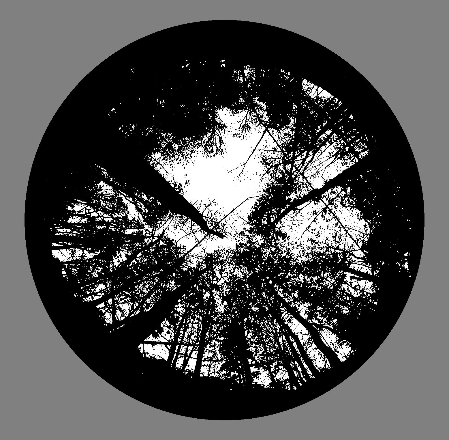
The circular mask (task 1).
The following images were all generated from the file norwayMaple-April-1W.pgm.
Using the "hand picked" method
Using ISODATA with "circle" regions
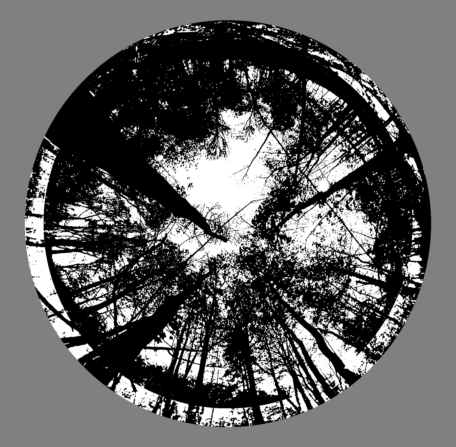
The outer-most region gets an abnormally low threshold from the ISODATA algorithm,
because it contains mostly dark pixels (trees, horizon, etc). Notice that
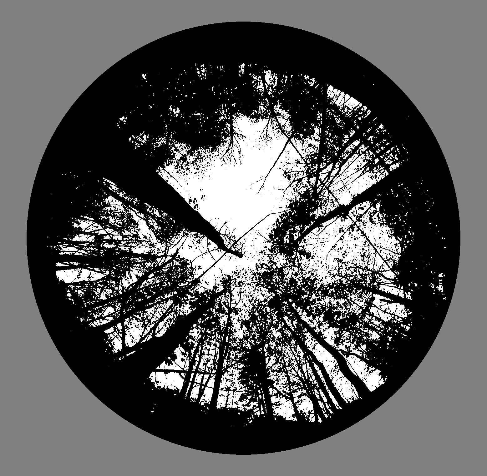
the "pie"-regioned image doesn't exhibit this flaw.
Using ISODATA with "pie" regions
Conclusions
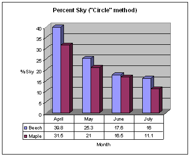
All three methods used give similar support to the hypothesis -- that the Norway Maple, being an invasive species, has larger leaves and leafs out earlier in the season, blocking out more light then. As the graphs above show, the Beech allows significantly more light through (larger % sky) than the Norway Maple in early months, but this margin decreases with time.
The Circle method shows this trend least well of the three, but most of this can be accounted for by the errors near the edges of the image discussed above.