Here is a small version without anti-aliasing.
In this lab, we extended our transformation library to be fully 3-D and implemented a viewing transformation function, and integrated it with our hierarchical modeling system.
In order to do a perspective projection, one must first define the viewpoint. The location where the virtual camera is placed is called the view reference point (VRP). The direction the camera is pointing is the view projection normal (VPN). Then a vector perpendicular to the VPN defines which direction will be considered "up" (VUP). Finally, the center of projection (COP) is the point through which all rays are projected in order to generate the perspective. To be physically meaningful, the COP should be place along the VPN in the negative direction.
Once the viewpoint is defined, the actual projection is just a series of matrix multiplications. First, the origin is translated to the VRP, and an orthonormal basis u, v is generated from VUP and VPN. Next, the origin is rotated to this basis, and then translated to the COP. If the COP is not along the VPN, a shear in z is done here to align them. Then the field of view (between the front and back planes) is scaled to the canonical view volume (CVV), which is defined as x = [-1, 1], y = [-1, 1], z = [0, 1]. Finally, we project onto the image plane using a perspective projection matrix, which is a function of d, the ratio of the z-distance between the COP and VRP in the CVV and the z-distance between the VRP and the back viewplane. To finish up, the appropriate reflections and translations are done to move to whatever image format is desired.
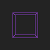
We demonstrate our perspective projection with a unit cube. First we have a single image of a view of the cube (COP) from the point (0.5, 0.5, -4) with the VRP at (0.5, 0.5, -2) and a view window size of (du, dv) = (1, 1).
Here is a small version without anti-aliasing.
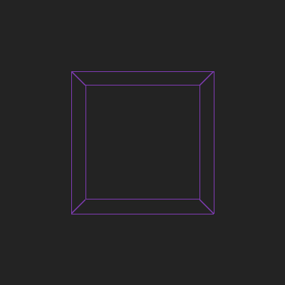
And here is a larger one with anti-aliasing.
We then extended our view of the cube by rotating it about two axes simultaneously and generated this nifty "tumbling cube" animation:
The cube! It tumbles!
The cop moves from a distance of 10 behind the VRP to 1.5 in front
of it and back.
The COP is always behind the VRP but translates along lines in a
clock-wise manner.